What you can do
You can find out how much of each number is your material and how much is your threshold. It takes two sets of runs against the API, and you can do it before you report anything.
The first set binarizes one gray volume at several thresholds.
- POST /api/v1/import-raw takes an 8-bit volume and a threshold, and returns the binarized structure.
- POST /api/v1/structures stores it, so every analysis below reads the identical voxels.
- POST /api/v1/metrics with includeTransportGraph gives porosity and the connectivity of the pore space.
- POST /api/v1/surface-area gives specific surface area, POST /api/v1/chord-length gives pore chord lengths.
- POST /api/v1/conductivity gives the effective transport number.
The second set is the yardstick. Generate the same recipe on several seeds and measure those the same way. That spread is what your material does on its own.
Then compare. Any quantity that your threshold moves further than the material does is reporting you, not the sample.
Why it matters
A threshold gets picked once and then never gets an error bar. It is chosen early, often by eye or by a default, and everything downstream inherits it silently.
Repeating the scan does not catch this. A second sample gives you a second number, and the difference looks like material variation whatever caused it.
So the question worth answering is not whether the threshold matters. It is how many gray levels of it your particular numbers can absorb.
They look like the same material
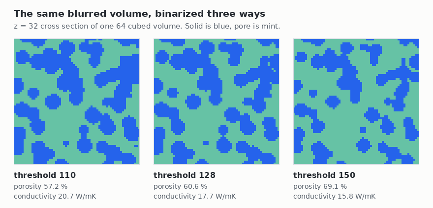
These three panels are the same z = 32 plane of the same volume. Nothing about the material changed between them. Only the threshold did.
The left and right panels disagree on effective conductivity by 31 %. Put them in front of a reader without the labels and nobody would call that two different materials.
The volume we thresholded
The gray volume is synthetic, and we made it that way on purpose. Starting from a structure whose answer we already know is the only way to say which threshold is wrong.
- PKR Core generated the base structure: the particle-packing example at 64³, 40 % target loading, 15 % overlap, on a fixed seed. Its porosity is 59.98 %.
- We read the voxels back and replaced them outside the API: solid became gray 200, pore became gray 50.
- We then blurred that with a separable Gaussian, mirrored at the edges, at two widths: sigma 0.8 and sigma 1.5 voxels. No noise was added.
- At sigma 0.8, 61.8 % of voxels land somewhere between the two levels. At sigma 1.5, 92.3 % do.
That blur is a stand-in for the partial-volume effect a real instrument produces. It is not a calibrated point spread function for any particular machine, so read sigma as "how many voxels wide is my transition band" rather than as an instrument setting.
Everything after this point is measured by the production API on that volume. The thresholds were 100, 110, 120, 125, 128, 131, 135, 140 and 150.
The yardstick: what the material does on its own
Five seeds of the same recipe, all thresholded at 128, give the honest spread. These are five different structures built to the same specification, which is the closest thing to five samples of one material.
| Quantity | Across five seeds | Span |
|---|---|---|
| Porosity | 60.42 to 60.59 % | 0.29 % |
| Specific surface area | 0.6490 to 0.6645 1/µm | 2.37 % |
| Mean pore chord, z | 8.75 to 9.30 µm | 6.09 % |
| Effective conductivity, z | 16.98 to 18.62 W/mK | 9.23 % |
The spread column is what matters. Porosity barely moves between samples, while effective conductivity moves more than thirty times as far.
That is not a flaw in the generator. Transport depends on where the narrow necks are, and that genuinely differs from sample to sample at the same loading.
One gray level buys very different amounts of error
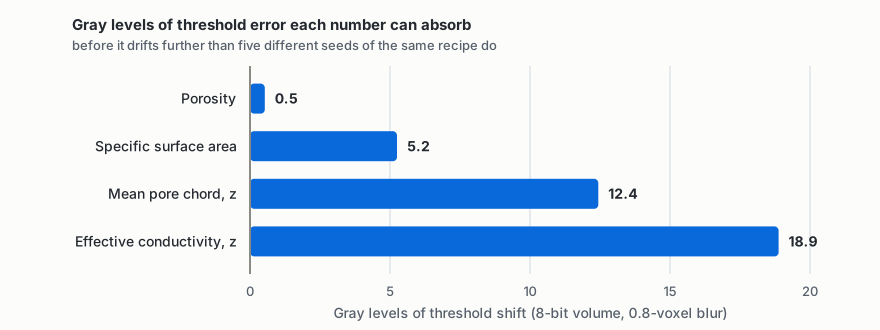
Porosity is the number the threshold ruins first. It takes about half a gray level to push it past the spread above, and a threshold is an integer.
| Quantity | Change per gray level | Gray levels it can absorb |
|---|---|---|
| Porosity | +0.55 % | 0.5 |
| Specific surface area | +0.45 % | 5.3 |
| Mean pore chord, z | +0.49 % | 12.4 |
| Effective conductivity, z | −0.49 % | 18.9 |
The middle column is the surprise. All four quantities respond to the threshold at almost the same rate, near half a percent per gray level.
What separates them is the yardstick, not the sensitivity. Conductivity moves just as readily, but it is judged against a far wider sample spread, so the threshold error disappears into it.
This inverts the usual worry. Porosity is the number people treat as a hard fact and transport is the number people treat as soft, and on this volume it is the other way around.
No single threshold gets everything right
You cannot calibrate your way out of this with one number. The threshold that recovers the true porosity is not the threshold that recovers the true surface area.
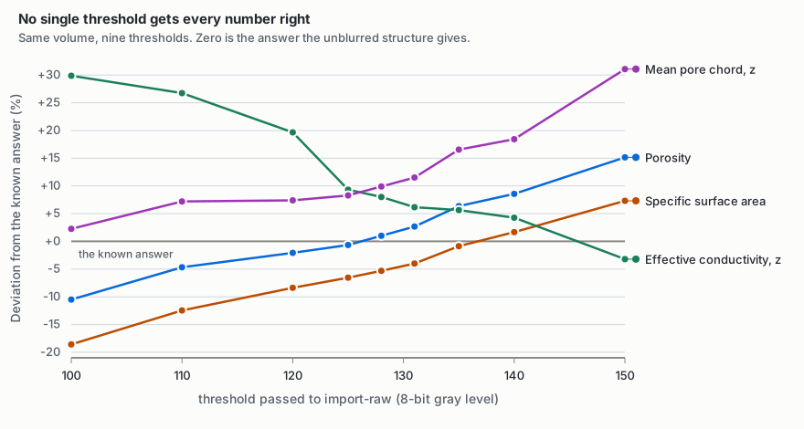
- Porosity matches the true value at a threshold near 126.
- Specific surface area matches near 137.
- Effective conductivity matches near 146.
- Mean pore chord never matches anywhere in the window. The closest it gets is 2.3 % high.
So picking the threshold that makes porosity exact has a price, and it is paid by the other numbers in the same report.
| Threshold tuned so that... | Porosity error | Surface area error | Conductivity error |
|---|---|---|---|
| porosity is exact (≈126) | 0.0 % | −6.1 % | +8.8 % |
| surface area is exact (≈137) | +7.1 % | 0.0 % | +5.2 % |
| threshold is the midpoint (125) | −0.7 % | −6.6 % | +9.3 % |
Read the first row against the yardstick table. A 6.1 % surface area error is more than twice the sample-to-sample spread, so no amount of extra sampling will reveal it.
The conductivity error in that row is 8.8 %, which sits just inside the 9.23 % sample spread. That is not reassurance. It means the error is there and you have no way to see it from the data.
A wider transition band rescales everything
Doubling the blur roughly doubles every rate. The ranking does not change, but the budget shrinks everywhere.
| Quantity | Per gray level at sigma 0.8 | Per gray level at sigma 1.5 |
|---|---|---|
| Porosity | +0.55 % | +1.00 % |
| Specific surface area | +0.45 % | +1.18 % |
| Mean pore chord, z | +0.49 % | +1.08 % |
| Effective conductivity, z | −0.49 % | −1.66 % |
This is the useful half of the result for anyone choosing an imaging setting. A sharper reconstruction does not make the threshold choice unimportant. It makes the same mistake cost less.
The one thing that did not move
Connectivity was immune. Across all eighteen blurred measurements the pore space kept a single cluster spanning z, at both blur widths and at every threshold.
- At least 99.98 % of pore voxels were in one component at every point.
- The count of z-spanning components was exactly 1 at every point.
- The lowest threshold at sigma 0.8 split the pore space into 14 pieces, but 13 of them were negligible.
There is a sensible reason. At 60 % porosity the pore network is far from the percolation threshold, so shaving the solid a little does not disconnect anything.
The lesson is about which questions are safe. "Is this connected" survives a bad threshold on this material. "How much of it is there" does not.
Running this on your own volume
You need your gray volume as raw 8-bit bytes and a list of thresholds. The loop below is the whole experiment for one threshold.
POST /api/v1/import-raw
{ "volumeBase64": "<your 8-bit volume>",
  "grid": { "nx": 64, "ny": 64, "nz": 64, "voxelSizeUm": 1 },
  "mode": "threshold", "threshold": 128, "materialId": 1 }
-> structure.voxels, structureSummary.statistics.occupancyRatio

POST /api/v1/structures
{ "structure": { ... } }                     -> structureId

POST /api/v1/metrics
{ "structureId": "<id>", "includeTransportGraph": true }
-> metrics.porosity
-> transportGraph.largestComponentFraction, transportGraph.through.z

POST /api/v1/surface-area
{ "structureId": "<id>", "materialId": 1, "method": "crofton13" }
-> surfaceArea.specificSurfaceAreaUmInv

POST /api/v1/conductivity
{ "structureId": "<id>",
  "request": { "version": "phase0.v1", "analysisType": "effectiveConductivity",
               "inputs": { "grid": { ... }, "materialProperties": { "1": 30 } },
               "params": { "direction": "z", "method": "graph-network" },
               "requestedOutputs": ["summary"] } }
-> value, meta.converged, meta.status- Store the structure once per threshold. Passing structureId to each analysis guarantees all five numbers describe identical voxels.
- Read meta.converged and meta.status on every conductivity call. A solver that did not converge should be a gap in your ladder, not a point.
- Build the yardstick from several seeds of one recipe, or from several real samples if you have them. Without it the threshold ladder has nothing to be compared against.
- Run the ladder on an unblurred volume first. If the nine points are not identical, something in your import path is wrong and the rest of the experiment is meaningless.
- The transport graph summary is capped at 64³ voxels, so run that part at or below that size.
What this does not settle
This is one recipe at one loading, in a 64³ box. A material near its percolation threshold would behave differently, and connectivity would almost certainly stop being the safe number.
The blur is isotropic and noise-free. A real reconstruction has noise, and often a point spread function that is wider through the stack than within a slice. Both would widen the numbers here rather than narrow them.
Conductivity was measured along z only, with the reduced graph solver. A full-grid solve would give different absolute values, though the threshold response is a property of the geometry rather than of the solver.