What you can do
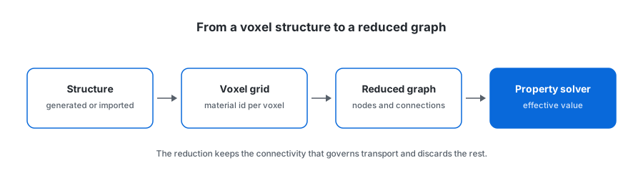
PKR Core can reduce a voxel structure to a graph — nodes for regions, edges for the connections between them — and solve properties on that graph instead of on the full grid. Several solvers offer this as a selectable method rather than a separate tool.
Why it matters
Effective transport through a porous structure is governed by connectivity far more than by the exact shape of every pore wall. Two structures with the same network of connected paths and different surface detail behave similarly; two with the same porosity and different connectivity do not. A graph keeps the first property and discards the second.
That is the whole trade. You lose the field — there is no per-voxel temperature or pressure map to look at — and you keep the effective value, computed on a problem orders of magnitude smaller than the grid.
The three tiers, and which is which
Where a property offers several methods, they are not competing implementations of the same thing — they answer at different resolutions.
| Property | Methods |
|---|---|
| Conductivity | simple, 3d, graph-network |
| Diffusion | effective-medium, graph-network |
| Permeability | pore-network, graph-network |
| Invasion percolation | graph-network |
| CO2 adsorption | graph-network |
| Elasticity | voxel-spring-network |
- simple / effective-medium — a closed-form estimate from bulk quantities. Instant, and blind to connectivity.
- graph-network — solved on the reduced graph. Fast, connectivity-aware, no field output.
- 3d — the full voxel field solve. Slowest, and the one that gives you a field to look at.
Note the asymmetry in that table: invasion percolation and CO2 adsorption exist only as graph-network methods. For those, the reduction is not an optimisation, it is how the problem is posed — percolation is a question about the connected network by definition.
When to use which
- Screening many candidates, or sweeping a parameter — graph-network. You want the ranking, not the field.
- Reporting a single structure you have already chosen — the full 3d solve, where it exists.
- Sanity-checking an order of magnitude — the closed-form estimate is enough.
- Percolation or adsorption questions — graph-network, because that is the only formulation offered.
The practical pattern is to sweep with the reduced solver, then re-run the two or three structures that survive at full fidelity. Doing it the other way round means spending the expensive solve on candidates you were going to discard.