What you can do
The web app is one client of the PKR Core API, not a privileged one. Anything the workspace does — generate a structure, analyze it, cut a cross section, sweep a parameter — is an HTTP call you can make yourself. That matters if you want PKR Core inside a notebook, a nightly job, or an agent loop rather than a tab.
- GET /api/v1/examples returns ready-made recipes, so nothing has to be hard-coded in the caller.
- GET /api/v1/materials returns the material constants, including thermal conductivity.
- POST /api/v1/generate builds the structure and, with storeStructure, keeps it server-side under an id.
- The analyses, the metrics, and the image export all accept that id instead of a fresh copy of the voxels.
One structure, uploaded once
A 64³ grid is 262,144 voxels. Re-sending that array with every analysis is what pushes a request body past the size limit, and it gets worse fast — 160³ is over four million. So the run registers each structure once with storeStructure: true and passes the returned structureId to everything downstream. The request bodies after the first are a few hundred bytes.
curl -X POST https://api.pakericore.app/api/v1/generate \
  -H "authorization: Bearer $PAKURI_TOKEN" \
  -H "content-type: application/json" \
  -d '{"recipe": {...}, "storeStructure": true}'
# -> { "structureId": "...", "structureSummary": {...}, "elapsedMs": 349 }
The three recipes come from GET /api/v1/examples with two edits: the grid is set to 64³ and the packings are raised to 45 % solid at 15 % particle overlap. The example recipes sit at 12 %, where the solid phase does not span the box and every effective property comes back as zero — a correct answer to an uninteresting question.
What came back
Eighteen calls, 10.3 seconds of wall clock for the whole thing. Conductivity is the reduced graph-network solver with a 30 W/m·K solid (Ceramic / alumina, from the materials endpoint); permeability is the pore-network solver.
| Structure | Generate | Solid fraction | Conductivity (W/m·K) | Permeability (µm²) |
|---|---|---|---|---|
| Particle packing | 349 ms | 0.450 | 19.21 | 0.258 |
| Fiber packing | 673 ms | 0.450 | 21.46 | 0.236 |
| Foam-like | 226 ms | 0.365 | 21.40 | 7.43 |
The foam is the odd one out in both columns, and for the same reason: its solid is one continuous phase rather than a pile of touching spheres, and its pore space is open. It carries slightly more heat than the packings despite being 8 points less dense, and it passes fluid roughly thirty times more easily.


A sweep, and its chart, from one request
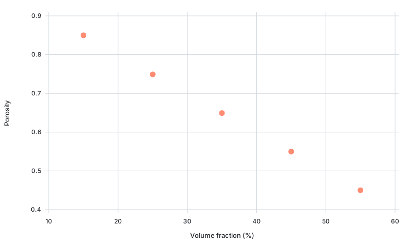
POST /api/v1/parametric-study takes a base recipe plus a list of overrides and runs the batch server-side. Asking for trendChart adds a standalone SVG to the response, so the caller gets a plot without a charting library. Five volume fractions from 15 % to 55 %, all five plotted, none skipped.
Where it stopped
The same run at 96³ is where the edges show. Generation stays quick — 1.0 s for the particle packing, 2.8 s for the fibers — and the pore-network permeability still answers, but the reduced conductivity solver has a ceiling on graph size and declines the larger structure. A reduced-order method buys its speed by working on a smaller object than the grid, and that object has a size beyond which the reduction stops paying for itself.
These numbers are what the reduced solvers returned, not ground truth. How far they can be trusted is a separate question, answered separately: the companion run checks the same API against cases whose answers are known in closed form.