What you can do
You can find out, for your own material, how large a box you have to compute before a single structure gives you a number worth quoting. Not from a rule of thumb, but from a scatter you measured. Sweep the seed at a fixed size to see how much of your result is the luck of one packing. Sweep the size to see where that luck stops mattering.
- One POST /api/v1/parametric-study builds up to 20 structures and solves each, so a ten-seed replicate set is a single request.
- Overrides change only the seed, or only the grid. The rest of the recipe stays fixed, so the spread you see is the structure and nothing else.
- Every case comes back in the response, so the mean, standard deviation and coefficient of variation at each size are yours to compute.
- trendChart returns the scatter as an SVG the server drew, ready for a report.
Why it matters
Box size is the per-sample cost of a dataset. When microstructures are generated in bulk to train a surrogate model, doubling an edge is eight times the voxels, so an old question gets asked again for a new reason: how small can you get away with?
The awkward part is that the answer is not a constant. It moves with the property, the phase contrast and the volume fraction, so a number from somebody else's material is a starting guess at best. What follows is not that number. It is the measurement that produces it.
Ten structures that were supposed to be the same
The recipe is the particle-packing example from GET /api/v1/examples, with filler raised to 45 % by volume at 15 % overlap so the solid phase percolates. The solid is the ceramicAlumina preset from GET /api/v1/materials, 30 W/m·K, against empty pore space. Conductivity is taken along z by the graph-network method. The grid is 48³ and stays there. Between the ten cases, only the seed changes — 1 through 10.
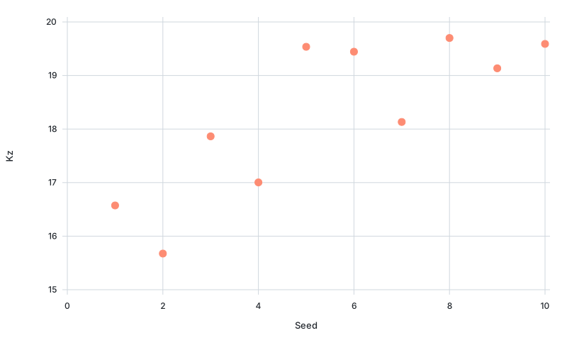
There is no trend in that plot, and there should not be: the seed is a label, not a parameter. What the plot shows is the size of the coin flip. Build one structure and report its conductivity, and the number you take away depends on which of these ten you happened to get. That is 4.03 W/m·K between the unluckiest and the luckiest.
The geometry was under control the whole time. The same ten structures reported porosities between 0.5479 and 0.5498, a coefficient of variation of 0.109 %. That is seventy times tighter than the conductivity measured on those very structures.
Here is the trap worth naming. A packing that hits its target fraction to three decimal places every time can still hand you an eight-percent scatter in transport. Confirming the volume fraction came out right says nothing about whether the conductivity has settled.
What growing the box actually buys
The same ten seeds then ran at six cube sizes. A study holds at most twenty cases, so sixty is six requests rather than one.
| Grid | Voxels | Mean Kz (W/m·K) | SD | CV | Min–max | Porosity CV | Request |
|---|---|---|---|---|---|---|---|
| 24³ | 13,824 | 19.50 | 1.795 | 9.2 % | 15.98 – 21.74 | 1.041 % | 1,275 ms |
| 32³ | 32,768 | 18.17 | 1.687 | 9.3 % | 15.42 – 20.28 | 0.345 % | 1,245 ms |
| 40³ | 64,000 | 19.24 | 1.181 | 6.1 % | 17.88 – 21.20 | 0.252 % | 1,997 ms |
| 48³ | 110,592 | 18.27 | 1.450 | 7.9 % | 15.67 – 19.70 | 0.109 % | 3,208 ms |
| 56³ | 175,616 | 18.93 | 0.801 | 4.2 % | 18.09 – 20.67 | 0.092 % | 5,017 ms |
| 64³ | 262,144 | 19.00 | 0.433 | 2.3 % | 18.37 – 19.72 | 0.037 % | 7,022 ms |
Read the CV column from the bottom up. At 64³ one structure sits within a couple of percent of the ten-box mean, so one box is a measurement. At 24³ it is within nine percent, so one box is a draw. The extremes are worse than the CV suggests: 15.98 and 21.74 W/m·K both came out of the same recipe. Porosity tightens too, and stays one to two orders of magnitude below the conductivity column the whole way.
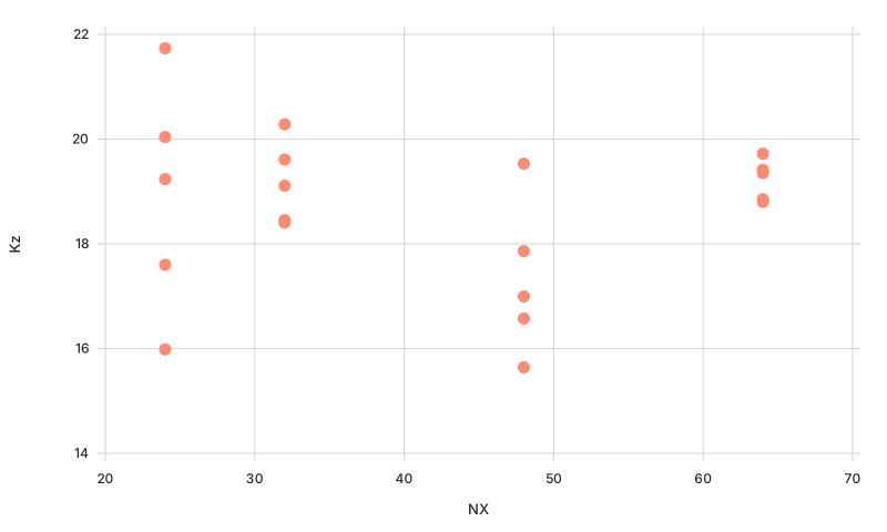
The means tell a different story from the spreads, and it is the more useful half. Going up in size they run 19.50, 18.17, 19.24, 18.27, 18.93, 19.00 W/m·K. There is no drift in either direction. They scatter by about as much as each mean's own uncertainty.
So the small boxes here are noisy, not biased, and that has a consequence. Ten boxes at 40³ took 1,997 ms altogether and pinned the mean to within about 2 %. One 64³ box costs roughly 0.7 s of the 7.0 s that ten of them needed, and pins it to within 2.3 %. Replicates at a modest size are the cheaper route to an average. What they cannot give you is one structure you can go on to crop, mesh, or hand to a full-field solver.
Running it on your own recipe
The request is a base recipe plus one row per replicate. The conductivity block is what makes the study solve rather than just build. Leave it out and every case comes back with geometry only, and a trend chart asking for conductivity.z plots nothing.
POST /api/v1/parametric-study
{
  "study": {
    "version": 1,
    "name": "Seed spread at 48^3",
    "baseRecipe": { "generatorType": "particlePacking", "seed": 1, "grid": { ... }, ... },
    "rows": [
      { "name": "n48-s1", "overrides": { "seed": 1, "grid.nx": 48, "grid.ny": 48, "grid.nz": 48 } },
      { "name": "n48-s2", "overrides": { "seed": 2, "grid.nx": 48, "grid.ny": 48, "grid.nz": 48 } }
    ],
    "conductivity": {
      "enabled": true,
      "method": "graph-network",
      "directions": ["z"],
      "materialProperties": { "1": 30 }
    }
  },
  "trendChart": { "xKey": "seed", "yKey": "conductivity.z" }
}
Every figure and number above came out of sixteen requests totalling 33.7 s.
One ceiling to plan around: the graph-network solver has a size limit. 72³ (373,248 voxels) returned 20.69 W/m·K. 80³ (512,000 voxels) generated fine and then reported conductivity as failed with graph_input_too_large. That arrives as HTTP 200 with the case marked success, because the refusal is on the analysis inside it. A batch runner has to read conductivity.directions.z.status rather than trust the status code.
What this does not settle
Ten seeds is enough to see a factor of four between the ends, and not enough to trust every step between. The CV column does not fall monotonically: 32³ came out no better than 24³, and 48³ worse than 40³. That is about what ten samples per size can resolve. Take the trend, not the individual rows. If you need the rows, run more seeds.
The solver adds a little of its own. The identical 48³ ten-seed request sent twice returned porosities matching to every digit, and conductivities that did not quite match: median relative difference 1.5 × 10⁻⁵, worst case 4.2 × 10⁻³. That is well inside the 7.9 % seed spread, so it changes nothing above. But if you are separating two candidates that differ by less than half a percent, it is the floor you work against.