What you can do
You can measure how much of your filler is in the one connected cluster that carries the property, before you commit to a loading. The number is a fraction of the filler you paid for, and it is different for every recipe and every dispersion.
Two calls on top of the structure you already generated are enough.
- POST /api/v1/invert swaps filler and void, which puts the filler phase where the connectivity summary looks.
- POST /api/v1/metrics with includeTransportGraph: true returns componentCount, largestComponentNodeCount and largestComponentFraction.
- The same response carries through.x / through.y / through.z: how many voxels sit in a cluster that reaches both faces of the box.
- One minus largestComponentFraction is the share of filler outside the biggest cluster.
What you do with the answer depends on which way it points. A high stranded fraction next to a conducting network says the loading is working but the dispersion is wasteful. A high stranded fraction with no spanning cluster says you are simply below threshold.
Why it matters
Conductive filler is expensive, and every extra point of loading costs processability and mechanical performance. So formulation work aims at the smallest loading that still percolates.
That target hides a cost. The threshold marks where something connects, not where most of your filler connects. Between those two loadings you are paying for material that sits in the binder doing nothing.
What was measured
One stock recipe, six loadings, four seeds each. The particle-packing example from GET /api/v1/examples was scaled to a 64³ grid at 1 µm per voxel, with spheres of radius 4 µm allowed to overlap by 15 %.
- Loadings of 15, 20, 25, 30, 35 and 40 volume %, on seeds 20260920 through 20260923.
- The generator hit every target: the worst gap between the requested loading and the solid fraction that came back was 0.10 percentage points.
- Conductivity along z came from POST /api/v1/conductivity with the graph-network method, with the filler set to 7 W/mK and the rest of the box void.
- Generating one structure took between 104 and 279 ms.
The connectivity split came from inverting each structure and reading the transport graph. POST /api/v1/cleanup-components was used later in the run, and the two agree on what a cluster is.
At 40 % loading on the first seed, the transport graph found 43 clusters holding 104,954 filler voxels, 99,988 of them in the largest. Cleaning up clusters below 4,096 voxels removed 42 clusters and 4,966 voxels, and left one. The two counts line up exactly.
The curve you get
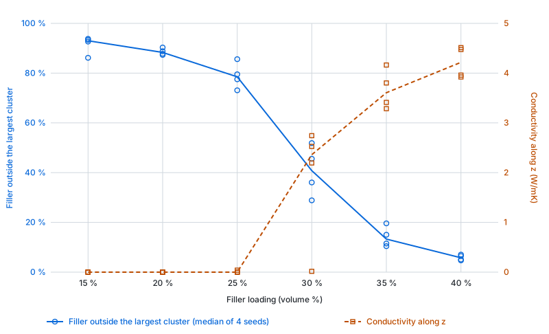
Stranded filler falls from almost everything to almost nothing across 25 percentage points of loading. The steep part sits exactly where the conductivity switches on.
| Loading | Filler outside the largest cluster, 4 seeds | Seeds with a z-spanning cluster | Conductivity along z (W/mK) |
|---|---|---|---|
| 15 % | 86.2, 92.7, 93.3, 93.8 % | 0 of 4 | 0, 0, 0, 0 |
| 20 % | 87.3, 87.8, 88.8, 90.3 % | 0 of 4 | 0, 0, 0, 0 |
| 25 % | 73.1, 77.5, 79.5, 85.6 % | 1 of 4 | 0.04, 0, 0, 0 |
| 30 % | 28.9, 36.0, 45.6, 51.9 % | 3 of 4 | 2.74, 2.53, 2.19, 0.02 |
| 35 % | 10.4, 11.5, 15.0, 19.6 % | 4 of 4 | 4.16, 3.80, 3.41, 3.29 |
| 40 % | 4.7, 5.1, 6.5, 7.1 % | 4 of 4 | 4.51, 4.48, 3.96, 3.92 |
At 25 % loading one seed in four returned 0.04 W/mK, which is half a percent of the 7 the filler itself carries. The first loading that returns anything real is 30 %, where three of the four seeds gave between 2.19 and 2.74 W/mK.
Those three had 54 %, 64 % and 71 % of their filler in the largest cluster. The median stranded fraction across all four seeds at that loading is 41 %.
Going from 30 % to 40 % loading buys most of that waste back. The median stranded share drops from 41 % to 6 %, while the conductivity of the seeds that conduct only rises from about 2.5 to about 4.2 W/mK. The last 10 points of loading buy little conduction, but they put nearly all of the filler to work.
The stranded filler is not dust
Almost none of it is speckle. POST /api/v1/cleanup-components removes every connected cluster below a voxel count you choose, and reports how many voxels went. Sweeping that threshold turns the cluster sizes into a distribution.
The sweep below is one seed at each loading, on the same structures as above.
| Loading | In clusters under 50 voxels | Under 250 | Under 1,000 | Under 4,096 |
|---|---|---|---|---|
| 15 % | 1.0 % | 11.3 % | 56.9 % | 100.0 % |
| 20 % | 0.7 % | 8.7 % | 43.9 % | 79.1 % |
| 25 % | 0.6 % | 6.3 % | 25.2 % | 48.4 % |
| 30 % | 0.5 % | 4.3 % | 15.7 % | 28.2 % |
| 35 % | 0.3 % | 3.5 % | 9.7 % | 15.0 % |
| 40 % | 0.3 % | 2.0 % | 4.7 % | 4.7 % |
Read the 30 % row against that seed, which had 36.0 % of its filler stranded. Clusters under 250 voxels account for 4.3 % of it. The rest of the waste is in clumps of thousands of voxels that never reach the main network.
A sphere of radius 4 µm is roughly 270 voxels at this resolution. So the stranded material is mostly groups of several particles that found each other and nothing else. Filtering out specks will not recover any of it.
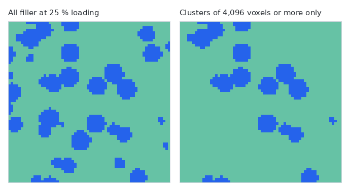
The endpoint caps that threshold at 4,096 voxels, which is why the right panel still holds four clusters rather than one. It is enough to see what is being thrown away, but it cannot isolate the largest cluster on its own.
Deleting it barely moves the number
The stranded filler carries almost nothing, and the conductivity says so. Every structure was analyzed again after the clusters below 4,096 voxels were removed.
| Loading | Filler deleted | Largest change in conductivity | Spread across the seeds that conducted |
|---|---|---|---|
| 30 % | 21.2 to 39.4 % | 0.34 W/mK | 0.55 W/mK |
| 35 % | 10.4 to 15.0 % | 0.21 W/mK | 0.88 W/mK |
| 40 % | 4.7 to 7.1 % | 0.27 W/mK | 0.59 W/mK |
At 30 % loading, deleting up to 39 % of the filler moved the answer by at most 0.34 W/mK. Changing the seed at the same loading moved it by 0.55. Three of those seeds conducted, so the comparison at that row is over three structures.
The changes went up as often as down. That is what you expect from material that was never in the path.
This is the part worth acting on. If a third of your filler can be deleted without the property noticing, the money spent on it is not buying conduction.
Running it on your own recipe
Generate once with storeStructure, then pass the identifier through invert and metrics. Nothing else needs to change in a recipe you are already sweeping.
POST /api/v1/invert
{ "structureId": "<from POST /api/v1/generate>" }

-> structureId            (the inverted structure, filler now material 0)

POST /api/v1/metrics
{ "structureId": "<inverted>", "includeTransportGraph": true }

-> transportGraph.nodeCount                  52438   filler voxels
-> transportGraph.componentCount               105   separate clusters
-> transportGraph.largestComponentFraction  0.1220   share in the biggest one
-> transportGraph.through.z                          voxels in a spanning cluster
The transport graph is computed for material 0, so the inversion is what aims it at your filler rather than at the pore space. Skip that step and you measure the pore network instead.
Size is the other thing to watch. The same request on an 80³ structure came back with a status of too-large and a stated ceiling of 262,144 voxels, which is 64³. Larger grids have to be coarsened first.
Run several seeds. At 30 % loading the four seeds here disagreed by 23 percentage points on the stranded fraction, and one of them did not percolate at all.
What this does not settle
This is one filler shape, one particle size, one overlap setting and one box size. A different shape, a spread of particle sizes or a different overlap will move the curve, and none of that was measured here.
The loading steps are also coarse. Five percentage points is a wide gap right where the curve is steepest, and the stranded fraction fell from 78 % to 41 % across one of them. Where exactly inside that step it happens is not something this run measured.
The two readings also disagreed once. One 30 % structure had no z-spanning cluster but still returned 0.017 W/mK, against a filler carrying 7. Near the threshold, treat a value that small as a hint to look at the connectivity rather than as a property.